When sharing, use this link.
In a prior paper (BARRETT11), I described the fundamentals of "Herringbone Wang Tiles", based on the traditional edge-constrained version of Wang Tiles. A note mentioned the possiblity of applying "corner colors" for Wang Tiles to Herringbone Wang Tiles. Implicitly, I was especially concerned with the application of "level generation", in which the generated tilings are examined closely by humans and want to have some specialized properties.
This follow-up paper explores several issues:
All the datasets examined in this paper (and a few more) have been made freely available (placed in the public domain). Additionally the C/C++ program used to generate the tilings (as well as to create the tile templates) has been library-ised and also placed in the public domain. Follow the link here.
In this section, I'll present some more results, and explore one aspect of the original result more closely.
BARRETT11 presented the results by expanding out to final image sprites, in this paper I will leave each image-sprite-tile as a single pixel in the image. This makes the results look "less cool", so it's important to keep in mind that the results we're looking at here are mainly about layout and connectivity, and not visual appeal.
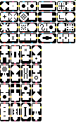
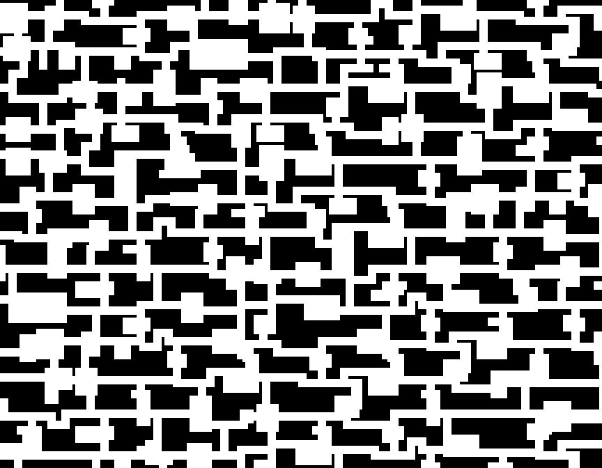
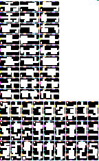
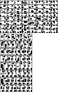
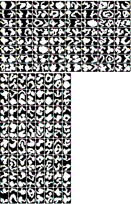
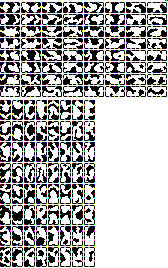
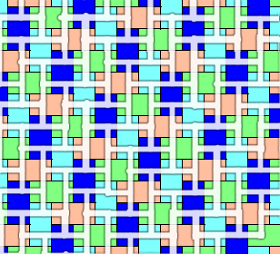
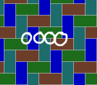
Here is the tile dataset from the original paper:
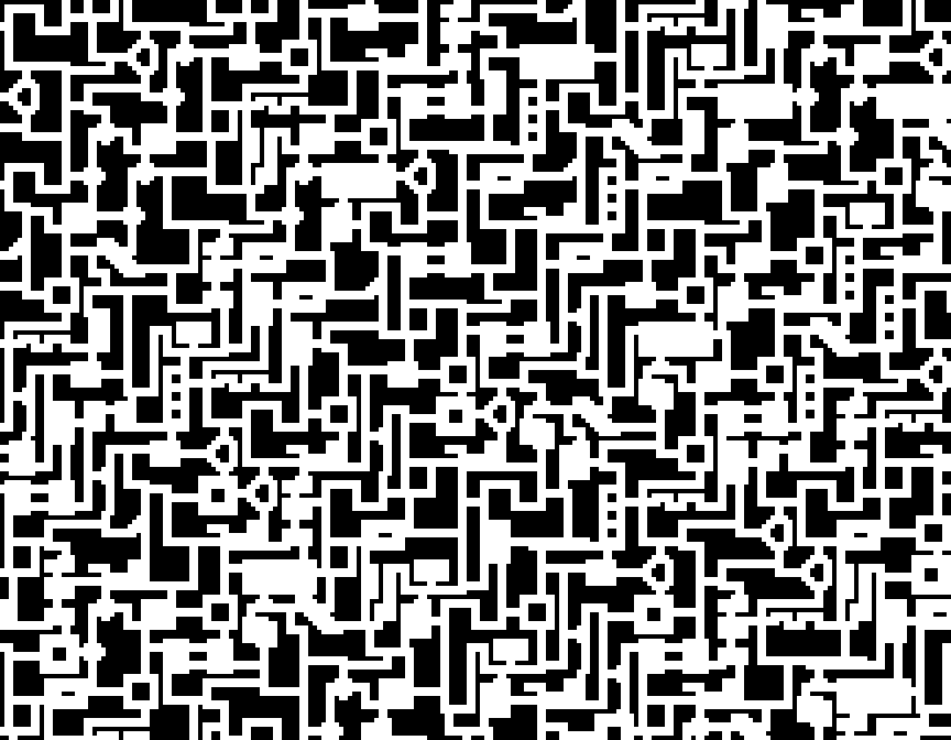
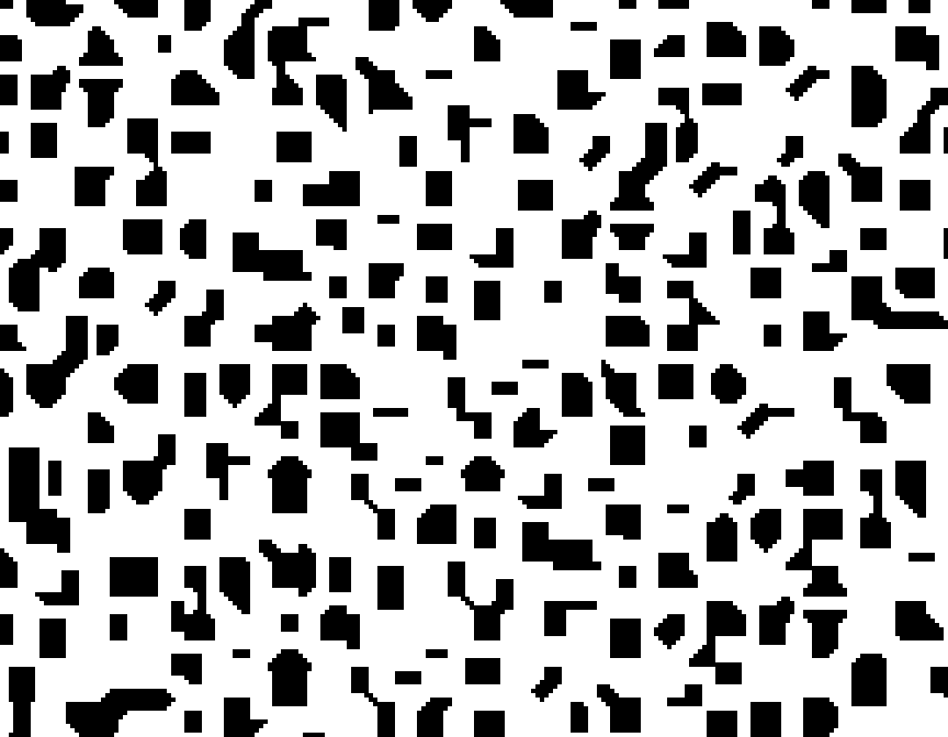
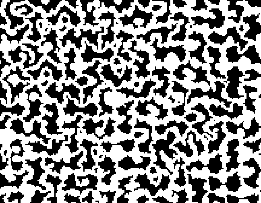
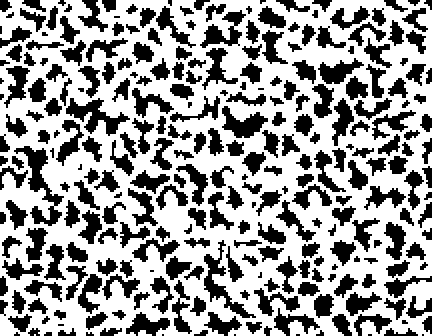
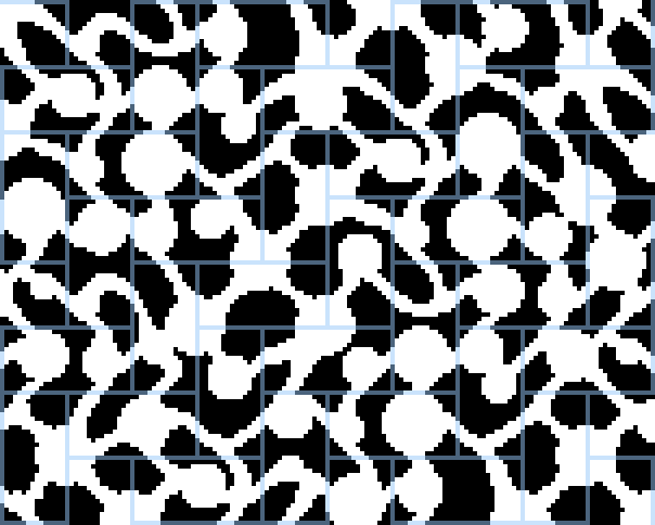
Here is a map generated from that tile dataset:
At this scale, and given the number of distinctive areas in the source data, it's easy to see repeating features. Whether this is acceptable to you or not is a design question. Additionaly, if each pixel were an "image tile" it's likely to be scaled very differently, and if there are procedural elements to the tiles it can be even less obvious.
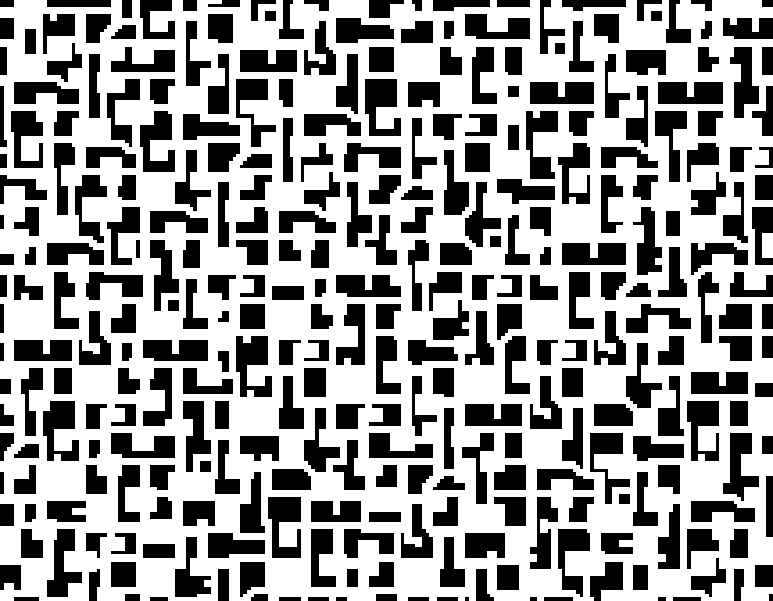
The above data set embraces the grid.
This data set shows significant bias along the herringbone diagonal.
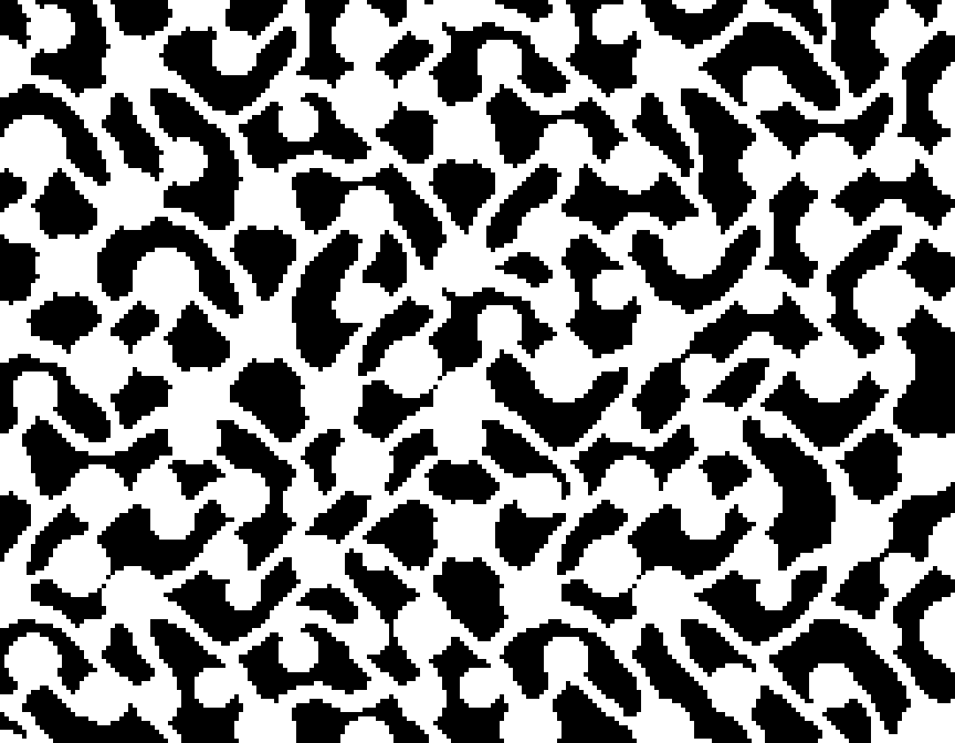

The above is heavily diagonals, but this is just due to the tile data, not the herringbone pattern. Note the seemingly free-form distribution of the circles.
This demonstrates how you can leverage the horizontal tiles to have have a horizontally-biased output; however, the herringbone diagonal is visible if you know to look for it.
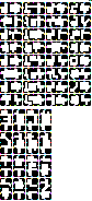
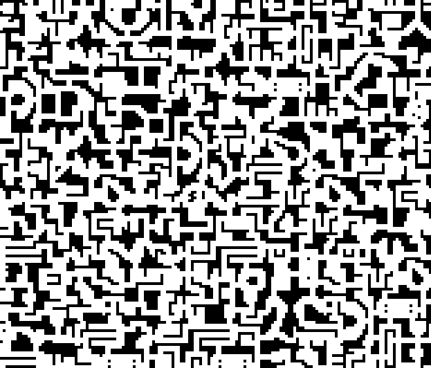
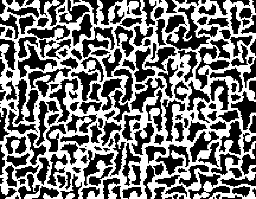
Following are three different approaches to caves. Note that the underlying grid is apparent (but probably unobjectionable) in the first two, but pretty much undetectable in the last one.
To explore this, I'll investigate in tedious detail some paths that illustrate the connectivity. To do this, we'll look at "right-hand rule" maze-followings, with dead-ends elimintated.
To explain: because of the way the data guarantees full connectivity, there are never dead-ends on a large scale (in the abstract connectivity graph), although there can be within-tile features that are local dead-ends. Instead, solid (unpassable) regions are always semi-locally bounded--they can never extend for more than a few tiles. (I.e., any white region is reachable from any other white region, but the black regions are divided into relatively small islands.)
This means that a right-hand maze rule will keep a single black island on its right the entire time, and will eventually loop around to its starting place.
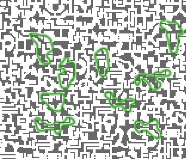
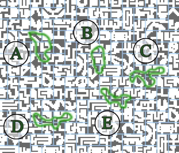
In this output, many of the loops are trivial, but some of the loops are more complicated, and in the following illustration I've marked some of them without regards to the underlying tile structure.
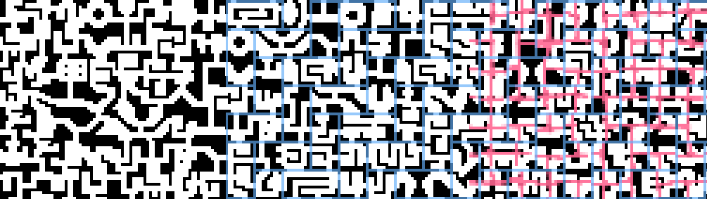
Let's focus on five of these paths:
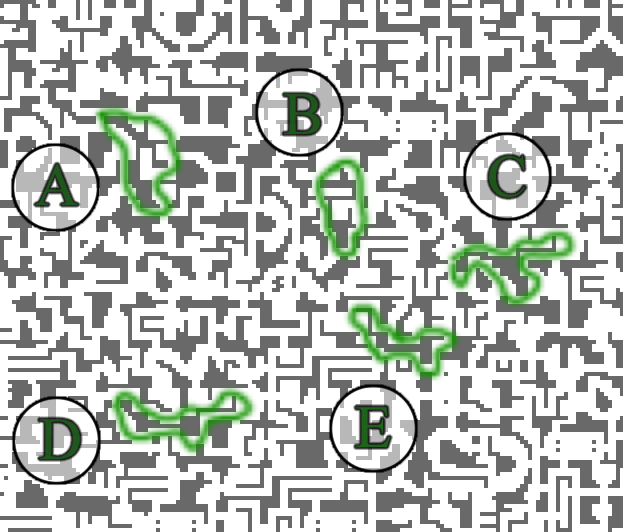
The marked paths can be described as:
This kind of variety of paths is why the connectivity seems complicated--especially when operating on a scale where a humanoid figure is about one map-pixel in size.
How does this dataset achieve this kind of complexity?
As explained in the previous paper, the core connectivity design is to fully-connect the edges in each half of a rectangular tile, but to only connect the two halves some of the time. With none of them connected, the abstract connectivity looks like this:
This doesn't actually seem very complicated, but this is largely a matter of scale. Let's look at the paths with the abstract connectivity of this tileset overlaid in red (keep in mind that the abstract connectivity lines are out of phase with the tile edges):
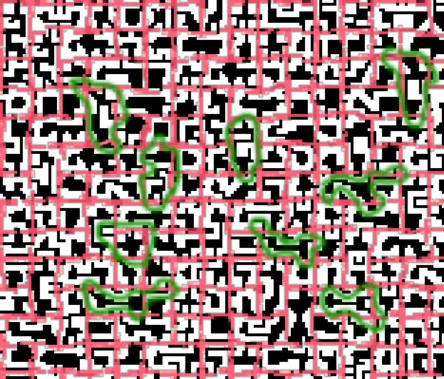
You can see here that every complicated path (except one) has a gap in the red lines representing the abstract connectivity; i.e., they are exploiting the intentionally-omitted connection between the two halves of each tile to create more complicated paths.
Moreover, you can see that the physical paths do not follow the abstract connectivity very closely, although they never deviate "too far"--for each segment of an abstract path that falls within a single tile, the corresponding physical path cannot leave that tile while still connecting the same endpoints.
To see that more clearly, let's look at the five paths in more detail by showing where the tile boundaries are:
(I have not bothered to also overlay the abstract connectivity because it looks too messy; you should be able to infer the abstract connectivity by remembering the basic rules of each half of the rectangle being fully connected.)
In every case, the basic pattern is a 3x2 or 2x3 half-tiles and 5 wang tiles. That is because this model of connectivity always has a worst case of involving 5 tiles. If a path from data created under this model required more than 5 tiles, it would mean there was an error in the data, and connectivity would no longer be guaranteed.
Using colored corners, we can actually do better than this, introducing more complicated connectivity in the abstract paths as well. This is the focus of section 3 of this paper.
This is a significant problem in something like texture synthesis or generating tile-based poisson distributions. In the "tile map" scenario we're mainly concerned with, this may not be objectionable; some of the maps shown in section 1 use edge constraints to no ill effect.
Lagae and Dutre also note a limitation of Wang corner tiles: they move the diagonal-adjacency problem described above to an edge adjacency problem; while Wang tiles do not meet cleanly at corners, Wang corner tiles do not meet cleanly at the center of edges, where data from the two corners collide.
Unwanted artifacts in the synthesized textures are typically located where patches meet. This is at the corners for Wang tiles and in the middle of edges for corner tiles. In this respect, Wang and corner tiles are similar. (LAGAE2006)
However, this analysis is not actually correct. The solution to this can be inferred from their section on poisson disk distribution generation. This poster (BARRETT12, published on twitter) sketches the idea, but I will describe it here explicitly.
Given C colors of corners, there are C unique corners, C2 uniquely colored edges (color pairs), and C4 uniquely colored tiles (color sets) in the full stochastic set. For those C2 unique edges, we can introduce redundant edge constraints, coloring each edge to be unique to those two edge colors. Then we can choose what data to display at the midpoint of that edge based on those constraints (same as we would with regular edge-colored Wang tiles), guaranteeing that the tiles match across that boundary:
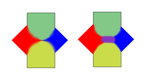
Here the green and yellow squares are Wang tiles that have been placed next to each other due to matching corner constraints, and the red and blue are both the corner colors and representations of where we fill in data from the corners in each tile. On the left, there is a discontinuity at the middle where four colors meet. (The problem is not that four colors meet, but that two colors meet across a tile edge, where their data has not been constrained to each other.) On the right, the discontinuity has been avoided by choosing specialized data for the edge. Note that the purple data must match across the two tiles, but this is the same constraint as is already true for the red and the blue. The only boundary-between-two-colors that the tile edge passes through are the corner-edge boundaries, but that boundary has been authored to be continuous above and below the tile boundary.
(I.e. the boundaries between each pair of colors may be generated through a stitching algorithm or human effort; but regardless all of them were explicitly generated offline.)
There is a similar issue for corners, which to be clear we will rename "vertices". Each rectangular tile has 6 vertices (four corners and two long-edge-midpoints). The vertices of the tiled plane can be grouped into four independent classes:
What this means for both edges and corners is that the colors of each class of edge/corner are actually independent. In Wang tiles, a red horizontal edge is unrelated to a red vertical edge (unless tile rotation is allowed). One can "rename" the colors of each edge orientation so they are totally non-overlapping without changing the tiles at all. Doing so is useful in practice when manually authoring herringbone Wang tiles, because it is important to not confuse one type of edge for another just because their geometric orientation is the same. Using distinctive colors avoids this.
It also calls attention to another degree of freedom in the Wang tile formulation. At first glance, a minimal stochastic Wang tile set that allows aperiodic tiling with random-access generation might seem to require 16 tiles: 2 colors for each edge and 4 edges, so 24. However, because colors for horizontal and vertical edges are independent, one can actually use 2 colors for horizontal edges and 1 color for vertical edges and create a tileset with only 2*2*1*1 = 4 tiles. (You can actually create aperiodic tilings using only two tiles, but those wouldn't make use of any Wang-tile-style constraints.)
This means I was incorrect in BARRETT11 when I implied the minimal "complete stochastic set" of herringbone Wang tiles was 2*26 tiles (64 horizontal and 64 vertical). Because there are 6 distinct edge types, it is possible to assign different numbers of colors to each edge type. For example, if all edge types that are horizontal get 2 colors, and those that are vertical get 1 color, then the number of horizontal rectangle tiles needed will be 2*2*2*2*1*1=16, while the number of vertical variants needed will be 1*1*1*1*2*2=4.
Similarly, the 4 kinds of herringbone corners can be assigned different numbers of colors. Each tile still has 6 vertices, so the math will look similar, but some vertex types appear more than once in a given tile.
In the above tileset, the number of colors per vertex type are (2,2,2,1). Because the 4th corner type appears twice in the vertical tiles and only once in the horizontal tiles, compared to the 64 tiles required for (2,2,2,2), horizontal tiles are 1/2 (32) and vertical tiles are 1/4 (16) as many.
In the above tileset, the number of colors per vertex type are (3,1,3,1). Both horizontal and vertical tiles have three vertices with three variants and three vertices with only 1 variant, so there are 27 tiles of each type.
The original dataset focused on a scenario of "dungeon"-like rooms and corridors. The approach chosen to map this onto herringbone Wang tiles (without any explanation) was to place rooms fully within Wang tiles, and to only allow corridors to cross the boundaries of Wang tiles. The connectivity model required connections between tiles along every edge, so there were a large number of corridors crossing the edges. The underlying assumption is that "rooms" need to be coherent and hand-authored, but corridors are generic and can transition across tile borders without being noticeable.
Given edge or corner constraints, it is also possible to place coherent human-designed features across tile boundaries, by designing those features once and copying the appropriate pieces to every tile with that constraint.
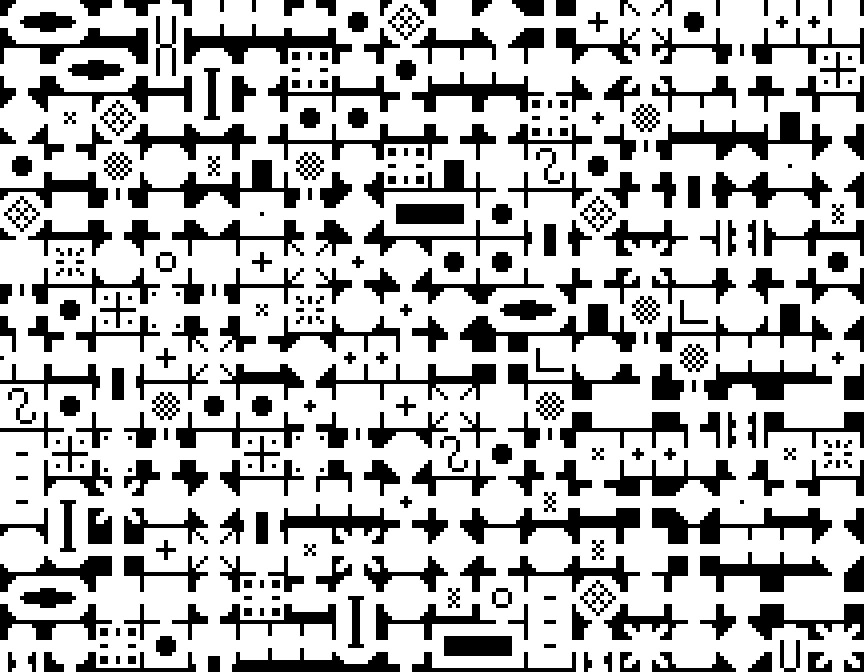
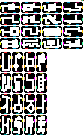
Consider for example this tile set from section 1:
You can see there are many circles that lie entirely within a tile, but you can also see that corridors meet at blobs in corners, which are actualy partial circles as well:
The upside of this approach is to better hide the underlying grid, since the circles aren't always within a single tile.
The downside is that the features are more homogenous; each "room" lying entirely within a tile can be unique, but each room lying on a corner needs to be identical across many tiles. For example, with 2 colors for every corner, 50% of tiles would have to have that same content in a given corner; and since each vertex type appears in 3 locations, something like 88% of tiles would need to have the identical feature somewhere on it.
In the above tileset, all the rooms are relatively homogenous circles (so the homogenity of the corner rooms is indistinguishable from that of the within-tile rooms), and the number of colors for each vertex are (3,1,3,1) to reduce the basic corner duplication from 50% to 33%. Only 2 of the 4 vertex types (the ones with 3 colors) admit rooms on their corners; you can see this in the output in that rooms-on-vertices only ever in a checkerboard pattern. (However, since there are so many non-grid aligned circles within-tiles, this is not obvious if the tiles are not explicitly drawn.)
Of course you can increase the number of corner colors to allow more room variation, but the number of tiles grows very rapidly as you increase the colors unless you only increase the colors of one corner, but this could introduce diagional artifacts.
A better approach would probably be to use corner colors but add content on edges. With 2 colors per corner, each edge actually gets 4 effective colors, which allows for more variety, and there are 6 classes of edges as opposed to only 4 classes of vertices.
In other words, with 2 colors for corners and 128 tiles, the amount of unique content allowed by each strategy is:
| Coloring | Feature placement | # unique content items |
|---|---|---|
| any | middle of (half-) tile | 128 (256 correlated) |
| corner colors | corners | 8 |
| corner colors | edges | 24 |
| edge colors | edges | 12 |
However, I have not yet explored placing features on edges; obviously mid-tile is a lot more inviting in terms of ROI of number of tiles to amount of content; the main reason to use edge content would be because the grid is too visible with only mid-tile content.
So it would seem you could have 18 unique pieces of content (6 edge types * 3 colors) compared to corner content which allows 6 pieces of unique content (2 vertex types * 3 colors), while only having 54 tiles (as in the round room example).
However, because each edge is adjacent to one 3-color vertex and one 1-color vertex, and each vertex is adjacent to three edges, it's actually the case that the three edges adjacent to each 3-color vertex are strictly correlated in their coloration, and thus any "unique" content placed on those edges will strictly vary together, thus appearing to be one piece of content not three pieces of content. This makes 18/3 = 6 effectively unique pieces of content, which is exactly the same as we get for placing content on vertices. (Which makes sense.)
Thus, if you wanted to explore using edge content while having fewer than 128 tiles, I might look at something like a (2,2,1,1) or (3,2,1,1) strategy where the vertices with multiple colors are adjacent to each other, thus producing edges that "really" vary. However, this probably causes unique content to be too obviously only along the herringbone diagonal.
(Note that in general for the type of full-connectivity we're concerned with, only the infinite plane is fully connected. It is possible with some strategies that if the map is truncated to a finite rectangle, some areas around the border will not be connected to the rest of the map. In the case of the strategy from BARRETT11 discussed in section 1, as long as the map truncation happens on tile boundaries, the only parts that may not be connected are cases where two half-tiles are not connected, one half-tile is off the map, and the content in the tile was intentionally shifted off-center so some of the content that is conceptually part of the off-map half-tile is not truncated: that content would only be connected to the off-map half tile, and so is disconnected in the truncated map.)
In section 2, I explained colored corners for herringbone Wang tiles. I also explored the possibility of placing "room" content on corners and edges. This would complicate the connectivity network model, so for this section, we'll return to the room-in-tile model, explicitly thinking of it as a network of vertices and edges connecting them. (Note that the vertices of the connectivity network are not the same as the vertices of the Wang tiles, and we will switch back to calling those "corners" to avoid ambiguity.)
A requirement of the connectivity model in section 1 was that every tile edge had a connection crossing it. This led to a highly-connected network, and most of the time only short paths are needed to get from one point to another point near it. (In some cases, as we showed, the paths were significantly longer, but the number of cases was low and the lengths were not enormous.)
In this section, we'll explore making use of corner constraints to reduce the very-high connectivity and to increase the length of the largest closed loops to e.g. cross 9 herringbone Wang tiles.
We'll use a similar strategy here; however, the starting point that will guarantee full connectivity is more complicated.
The basic model we'll take, given that we're using colored corners, is to make each corner responsible for guaranteeing that the four half-tiles immediately surrounding that corner must all be connected.
This guarantees that every half-tile is connected to every other half-tile: between any two arbitrary half-tiles, you can find a path of orthogonally-connected half-tiles between them, and then the corners adjacent to each pair of half-tiles in the path guarantee connectivity between those two half tiles; each pair in the path is connected, so transitively the ends of the path are connected.
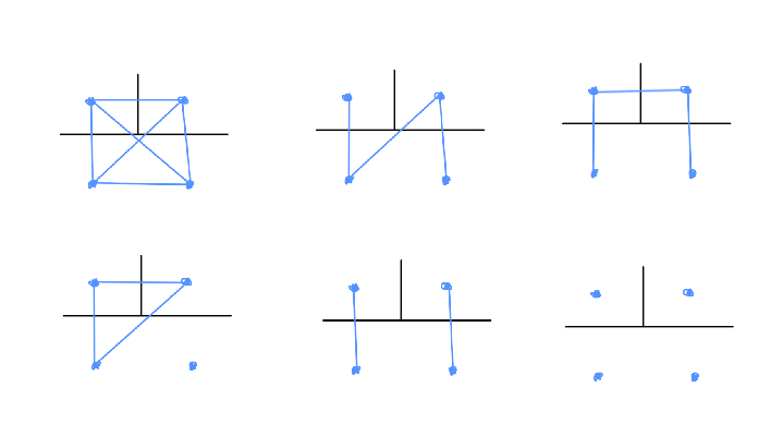
In the top row, all four vertices are fully-connected; there is some indirect path between any pair of vertices. In the bottom row, all the vertices are not fully-connected; it is impossible to get from some vertices to some other vertices.
The original method in BARRETT11 actually corresponds to using the pattern at the top right, in which every tile edge has a connectivity edge passing through it, but there doesn't need to be one through the center of the tile. Since every vertex is (at least indirectly) connected to every adjacent vertex, the tiles were all guaranteed to be connected.
The trick we're going to use with colored corners is to treat the four types of corners differently. We will guarantee map connectivity in the same way: any two adjacent vertices must be (at least indirectly) connected because a nearby corner guarantees it. However, the way those corners guarantee it will be different for the four corner types.
Specifically, we will use induction on corner types. Type 1 will guarantee it outright; type 2 will guarantee it by relying on the the guarantee for type 1 corners; type 3 will rely on type 2 & type 1, and etc.
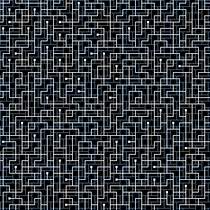
Note that there are cases where shortest loops must cross as many as 9 or perhaps 10 tiles.
Half-tiles with only one incident network edge are marked with special terminal nodes. However note that there are only two directions from which those edges come (the termination occurs while travelling left or up, never right or down). This is a limitation of the chosen strategy.
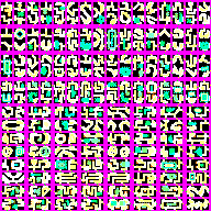
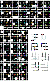
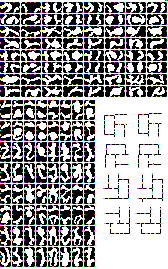
Here is the data set used to generate the above:
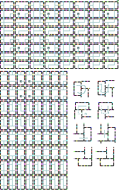
Here is the induction used to guarantee connectivity:
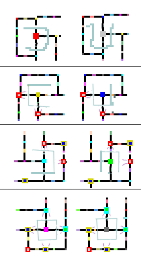
The first type of corner is colored either red or grey. The pale teal lines show what network connectivity is explicitly added in the form of connections across the edges. The U-shape is used as shown earlier since it guarantees all four vertices are connected. (Two different connection strategies are used to add variation, but this does not affect the connectivity overall.)
For the second type of corner, colored yellow or blue, we can see that there are adjoining vertices that are red-or-grey. The corner on the left guarantees that the four vertices around it are connected; that guarantees that the lower-left and upper-left vertex around this blue/yellow corner is already connected. We draw in a thin teal line to show that they are already (indirectly!) connected. Similarly, we draw in a thin teal line below the corner because of the guarantee from the red/grey corner below that.
With two network connections already guaranteed, we only need to add one explicit edge to guarantee all four vertices are connected. Again, we use two different choices to guarantee variety.
For the third type of corner, we again get two guaranteed connections due to the presence of red/grey corners. (There are also blue/yellow corners nearby, but they are only on diagonals and thus don't guarantee the connectivity of any of the adjacent vertices). Again, two edges are implicit, and so we only need to add one new edge.
For the fourth type of corner, every adjacent corner is of a type that has already been inducted, so every vertex around the corner is already fully-connected. Thus no network edges need to be introduced.
Of course, in every case, we can always add non-required edges, by using edge colors to make the choice consistent across all tiles.
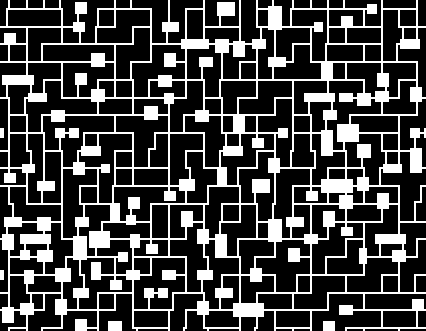
As can be seen if you animate between them, these two maps use almost the exact same connectivity (the same one defined above):
and they produce the following plane tilings using the same random number generator so the same tile layout:
The caves here show complicated connectivity but are more obviously aligned to the grid than some of the alternatives shown in section 1 (which for example put features on corners).
It seems like the approach shown in the previous subsection is "overly connected", since the fourth type of corner already had one more guaranteed indirect connection than it needed. A strategy which might be able to reduce this would be to induct over sides-of-corner-types instead of over corner types. For example, you might first guarantee that the two vertices to the left of corner type 1 are connected by putting in an explicit connection. Then, instead of guaranteeing the other sides of type 1 (as the previous did), you then guarantee connectivity some other side of some other type, one which can leverage the left-of-type-1 guarantee. Iterating through the 16 combinations of types&sides in an arbitrary order, you may be able to reduce the number of mandatory edges, or at least make the results more symmetric.
Note that all of this only matters if you want to try to control connectivity in the authoring of the herringbone Wang tile data. As mentioned in BARRETT11, it is not hard to write a "dungeon generator" which explicitly keeps track of connectivity and makes sure everything is connected. By placing "procedural connections" in tiles (which the engine knows how to make present or absent), program code can explicitly manage the connectivity even when using Wang tiles. Additionally, program code can make global connectivity guarantees, or allow maze-like connectivity where there is only a single path between any two points. These sorts of constraints can not be achieved using Wang tile design.
A number of algorithms and techniques arise with herringbone Wang tiles because there are six distinct "edge orientations" and four distinct "vertex types". One can achieve similar effects with regular Wang tiles by introducing such edge orientations and vertex types artificially. This allows you to do things like create complex connectivity directly in the data, or forbid a tile from ever appearing right next to itself (although only by quantizing where each tile can appear; e.g. if you make the corner type derive from the bottom bit of x and y, then each tile can only appear in, say, odd columns and even rows).
Of course, if we have a Wang tile set with four corner "types" each having two colors, this is exactly the same as a Wang tile set with one corner type each having 8 colors; the difference being that the full-stochastic-set for four-types-two-colors is not a full-stochastic-set for 8-colors. The full stochastic set in the first case has 24 tiles since each corner is one of two colors, while the latter would have 84 tiles. If you're using Wang corner-colored tiles and using an algorithm that assumes the full stochastic set (e.g. it allows random-access by pseudo-randomly coloring each vertex), you can't directly use this technique. However, it's not difficult to modify the algorithm: with two colors per corner, the effective color at each corner uses 1 pseudo-random bit and 2 non-random bits which are structured in a way to guarantee an appropriately-colored tile exists.